Frenzied Flow

“My job is to break the model,” says Kathy Prestridge.

An aerospace and mechanical engineer by training, Prestridge spends her days attacking one of the Lab’s most foundational scientific challenges: predicting the motions of fluids. The model she refers to is a collection of equations, computer codes, and best-fit approximations governing the behavior of fluids under extreme conditions, like those deep inside a nuclear weapon, a fusion reactor, or a star. She’s on a mission to understand fluid flows and reveal the model’s flaws.

Fluid dynamics, or the motions of liquids and gases, manages to be unexpectedly baffling, even in everyday situations. When a fluid flows smoothly, it can be understood by mathematically dividing it into a stack of parallel flows, as if the fluid passed through an egg slicer. But when a flow is just a little more energetic, it can become turbulent, churning and swirling in unpredictable ways. The difference is like that between an ocean wave rolling and an ocean wave crashing.

Even for something as pedestrian as pouring cream into coffee, the equations that govern the fluid dynamics are simply too difficult to solve, even with a powerful computer. Little motions that deviate from computer-model predictions quickly balloon into eruptions and vortices that can end up dominating the whole flow. In fact, some scientists would argue that more is known about the interior of a black hole—a region where no experiments have ever been conducted and, even if they were, their outcomes could never be observed—than about cream mixing into coffee. Or smoke from a snuffed-out candle. Or a gust of wind.

Despite decades of effort to remedy this deficiency, models of turbulent flows, especially those in extreme environments, still don’t capture all the relevant physics. Hence Prestridge’s desire to break the model: she must find where the current model fails so that it can be fixed or improved—or at least have its weaknesses properly identified. And just recently, she succeeded. She broke the model. Twice.

What little whirls are made of

Much of human understanding of turbulence derives from a 1941 theory by Andrey Kolmogorov (the “K41” theory). He described a turbulent flow by adding to a large-scale flow velocity (e.g., the overall flow of a river) a bunch of smaller-scale velocities (e.g., patches of whitewater). The idea was that whirls of fluid, called eddies, would spin off from a turbulent flow, siphoning energy away from the original flow to do so. As one eddy pushes into the surrounding fluid, it spends its energy spawning other, smaller eddies, which produce still smaller ones after that. Eventually, far enough down the chain, a great many tiny eddies combine to produce fluid moving in every direction equally—a property known as isotropy. These isotropic movements ultimately give their energy to movements on the molecular scale, generating heat according to the viscosity of the fluid. The heat then dissipates into the surrounding environment. Another early contributor to turbulence theory, Lewis Fry Richardson, in the book Weather Prediction by Numerical Processes, put it this way:

Big whirls have little whirls that feed on their velocity, and little whirls have lesser whirls and so on to viscosity.

Early models of turbulence adopted the K41 big-whirls-little-whirls paradigm, and many modern models are still based upon that foundation. The trouble is, detailed measurements reveal that it’s not actually true for many of the flows that are important to Los Alamos research. Small-scale fluid motions produced by the cascade of whirls are not isotropic, not even on average. And as Prestridge’s team would discover, the energy doesn’t always flow from larger whirls to smaller ones. The reality is much more complex, but it takes some serious advanced-measurement capabilities to see it.

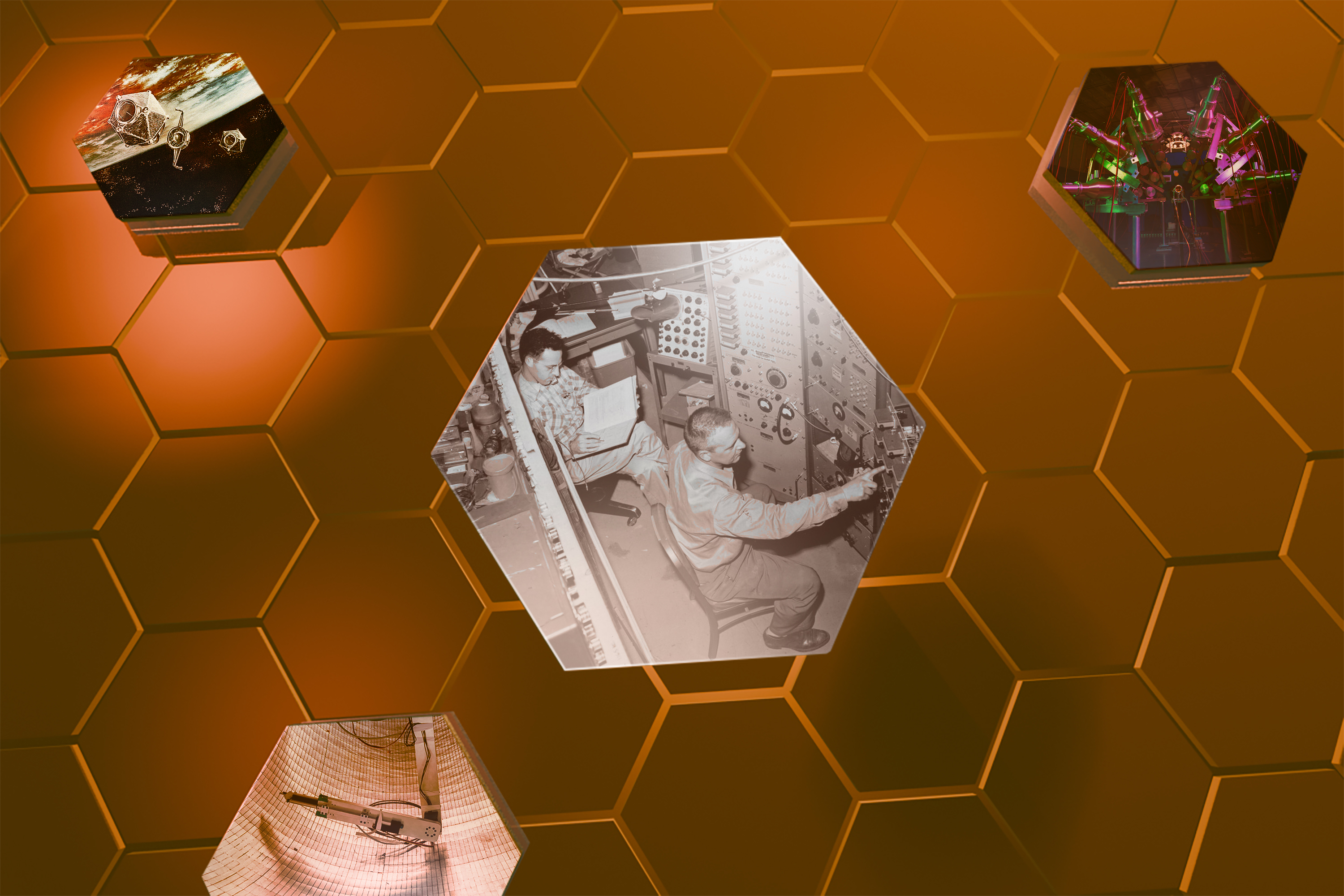
It takes some serious advanced-measurement capabilities to see what really happens

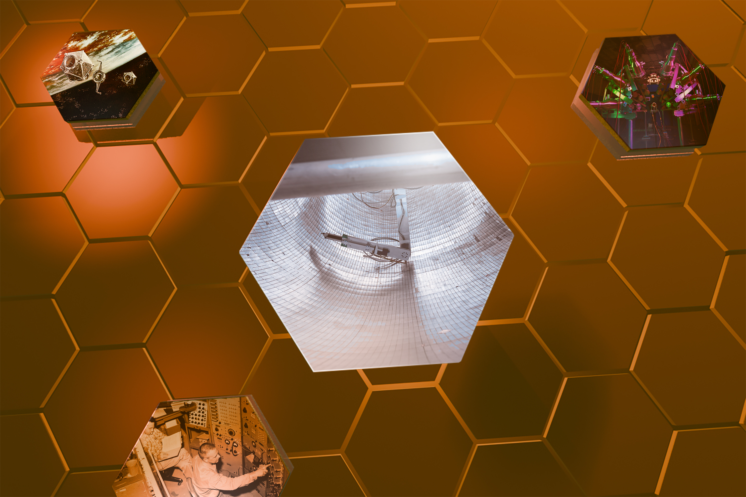
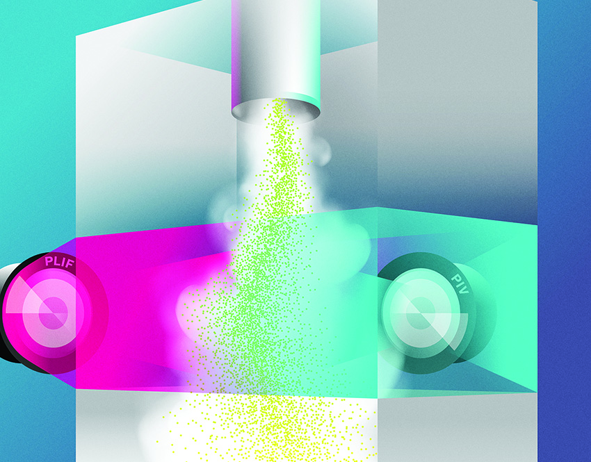
Prestridge’s research facility includes a turbulent mixing tunnel—in which a downward-pointed jet of fluid emerges from a pipe into a surrounding fluid—instrumented with technology that’s the envy of the fluid-dynamics community. First, she uses planar laser-induced fluorescence (PLIF), which, after an initial laser measurement and a great deal of subsequent mathematical analysis, provides a detailed map of the variations in fluid density throughout a wide horizontal band spanning the jet’s wake and the surrounding fluid. It subdivides that band to a resolution of 41,000 tiny patches of fluid. On top of that, she uses particle image velocimetry (PIV) to track the motions of microscopic tracer particles in the flow. A pair of back-to-back images shows how the particles move in a very short time, allowing Prestridge to compute their instantaneous velocities. That allows her to assign a tiny, unique arrow to each of the 41,000 patches of fluid, in addition to each patch’s PLIF-derived density.

In previous experiments throughout the research community, it was always either-or: PLIF for densities or PIV for velocities, but not both. The only way to get both was to do the experiment twice. But because turbulence is notorious for producing inherently random variations from one trial to the next, researchers couldn’t assume that the observed densities actually corresponded to the observed velocities. Now, in Prestridge’s experiments, they can. Densities and velocities are measured together in all the same patches of fluid at the same instant. This means, for the first time, she has detailed information on all the small-scale motions across the flow. It is no longer necessary to assume it’s isotropic.

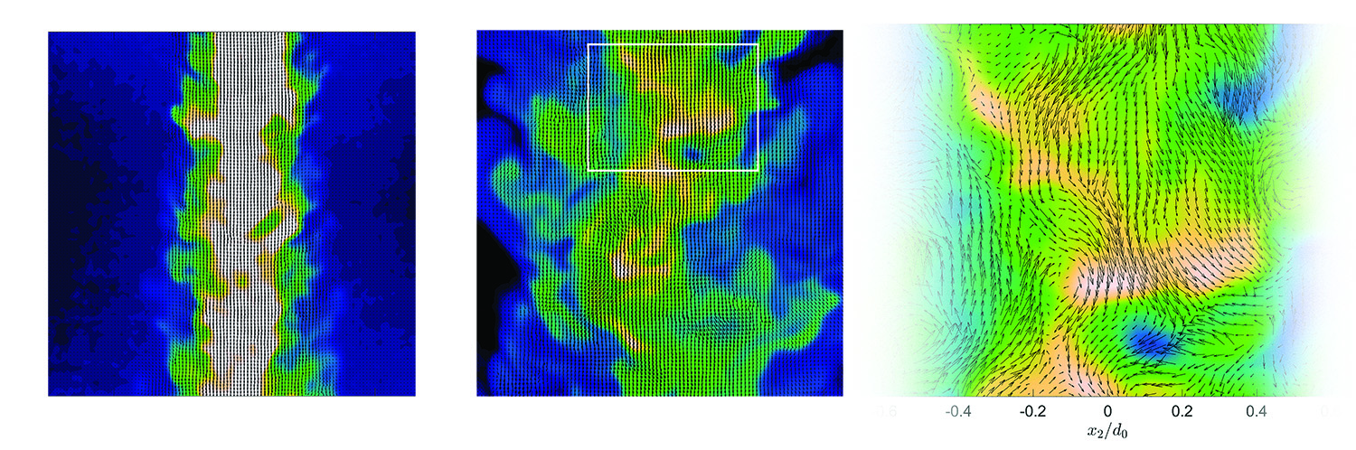
More than that, Prestridge and her team take all three images—one PLIF and two back-to-back PIVs—10,000 times in succession during each trial to obtain comprehensive statistics on the densities and velocities of the fluid as conditions vary within the turbulent flow. That’s three high-resolution measurements taken 10,000 times across 41,000 discrete locations in the flow, for anyone keeping count. And they do all that at multiple locations downstream from where the jet emerges from the pipe. Then they do the whole experiment again with a different fluid.

What big whirls are made of

The initial experiment involved a stream of air, laced with tracer particles, exiting the end of a pipe into a tunnel also filled with flowing air. This type of experiment is consistent with the “Boussinesq approximation” often made in fluid dynamics: that there is effectively just one uniform fluid, in this case air, rather than multiple fluids with different densities mixing. (The approximation is useful, for example, when considering ocean currents and not wanting to get bogged down with variations in salt content from one patch of seawater to the next.) The air-on-air Boussinesq flow experiment yielded rich PLIF and PIV data sets, but the major surprise came from Prestridge’s subsequent non-Boussinesq flow experiment.

In that experiment, a stream of sulfur hexafluoride— an inert, nontoxic gas four times denser than air—entered the air-filled tunnel. This time, the data revealed a previously unobserved phenomenon called “negative production of turbulent kinetic energy” (TKE), which utterly upended the prevailing K41 paradigm. It meant that, near the centerline of the flow, small-scale eddies were delivering energy to large-scale fluid movement, instead of the other way around. Subsequent analysis revealed that the small-scale eddies were actually deforming and stretching into larger eddies—a mechanism for transferring energy that’s not included in K41. Being the first to conduct an experiment with strong density gradients and simultaneous, fine-scale, across- the-flow density and velocity measurements, Prestridge’s team was the first to observe the effect.

The implications are striking. More than just a curiosity, negative production of TKE is evidently an essential aspect of non-Boussinesq flows and one not accounted for in current models and codes. Moreover, the effect would be amplified in extreme pressure, temperature, and density conditions— as in the nuclear-driven flows studied so extensively at Los Alamos.

“Right off the bat,” says Prestridge, “it is critical to figure out if there’s something new here that our scientists need to know about turbulent flows when a nuclear weapon is detonated.”

Yet it’s not just about nukes. Fusion-energy technology, in particular, is vulnerable to complications from turbulent fluid dynamics, and there are many possible reasons why “ignition”—a self-sustaining fusion reaction that generates more power than it consumes—remains elusive at advanced facilities, such as the National Ignition Facility (NIF) at Lawrence Livermore National Laboratory.

All the models predict slower-moving particles than what you get in real life

“The strong density gradients and shocks present in NIF experiments are likely to induce all sorts of mixing,” says Prestridge. “It’s difficult to resolve with our codes and predict with our current models.”

Turbulent mixing effects are everywhere, and, in a way, even the elemental makeup of the universe hangs in the balance. Many chemical elements are created during the supernova explosions of white dwarf stars. These stars may well have deep plumes of stellar matter with complex mixing under the surface just prior to detonation, causing non-Boussinesq dynamics to influence the outcome. If scientists can’t predict the dynamics of the explosion, they will also be unable to predict the abundances of the elements blasted into space or the corresponding chemical evolution of galaxies. This makes astrophysicists very interested in turbulent flow models.

Another shock

Not one to be satisfied with merely breaking a turbulence model central to nuclear technology and exploding stars, Prestridge went ahead and broke another. This time, her target was particle acceleration induced by drag from a passing shock wave. A shock wave is supersonic, and naturally, being hit with one represents a distinctly unsteady type of flow. This contrasts with the steady flows normally studied to predict drag on objects such as airplanes or golf balls.

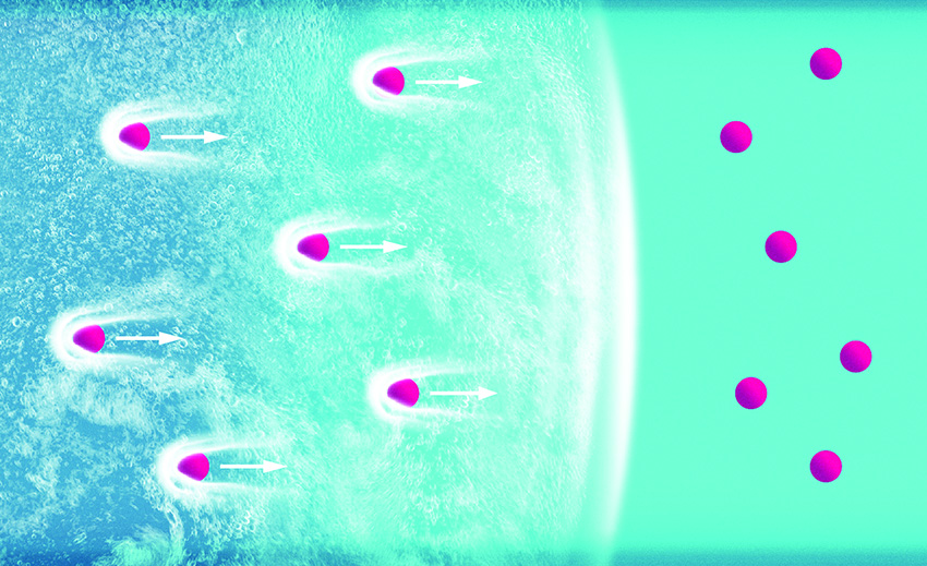
Prestridge’s team suspended micron-sized (millionth of a meter) spherical particles in air within an apparatus called a horizontal shock tube and then sent a shock wave down the length of the tube. The particles, initially still, accelerate sharply in response to the passing shock, chasing it down the tube. The rushing air drags the particles forward, similar to a leaf being whipped up in the wind or, in reverse, a skydiver reaching terminal velocity. A drag coefficient is used to quantify the strength of the drag, and, wouldn’t you know it, Prestridge discovered that the drag coefficients in the models were all wrong. In particular, they were too small.

“The steady-flow models and the only partly relevant unsteady-drag models out there get it wrong,” says Prestridge. “The accelerations they predict are too low, meaning that their predictions yield slower-moving particles than what you get in real life.”

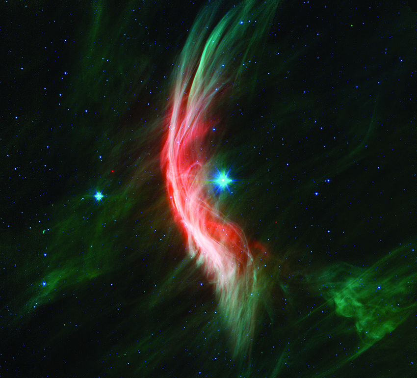
Not surprisingly, bits of shock-accelerated particulate matter creep up in a lot of the same settings where the behavior of non-Boussinesq flows is important, including nuclear technology and astrophysics. For example, for many energetic astrophysical phenomena, such as expanding supernova remnants, it is valuable to predict how dust particles will move in the presence of a shock wave.

New modeling will have to accommodate the non-Boussinesq flow and unsteady-drag data so that computational fluid dynamics codes can be updated, science advanced, and technology improved. Fortunately, at Los Alamos, Prestridge is able to collaborate with colleagues doing a variety of experimentation, simulation, and modeling, all in one place. So after breaking the model, she can also have a hand in fixing it.