VALIDATION OF THE ACCURACY OF THE LABSOCS MATHEMATICAL
EFFICIENCY CALIBRATION FOR TYPICAL LABORATORY SAMPLES
Frazier
L. Bronson CHP Ram
Venkataraman Ph.D.
fbronson@canberra.com rvenkataraman@canberra.com
Canberra
Industries, Inc. 800 Research Parkway Meriden CT USA
Presented at the 46th Annual Conference on
Bioassay, Analytical, and Environmental Radiochemistry.
November 12-17, 2000 Seattle, Washington
LabSOCS [Laboratory Sourceless Object Calibration
Software] is a computer program that performs mathematical efficiency
calibrations of Ge detectors, without any use of radioactive sources by the
laboratory user. This allows quick and
accurate calibrations of many geometries that are difficult to do [non-water
samples], take time to obtain the reference sources and make them simulate the
sample, require radiochemistry
knowledge to make the simulation accurate, and cost money to purchase the
radioactive calibration standards and pay for the labor. Thus, the advantages of an accurate computer
program to do this are obvious. The
purpose of the tests summarized in this document is to show how accurate the
mathematical calibration is.
The LabSOCS software is an improved version of the
successful and widely accepted ISOCS [InSitu Object Calibration Software]
mathematical in-situ efficiency
calibration product. The improvements
relevant to laboratory applications include a totally revised detector
characterization method for increased accuracy at very close distances, new
computational algorithms to improve attenuation corrections at close energies,
and also a method to better describe the contour of a complex beaker shape for
improved accuracy.
To show the accuracy of the calibration method, several
documents are provided to the user.
First is the "Validation and Internal Consistency" document,
containing the results of 120 intercomparisons between ISOCS/LabSOCS and a
reference method. For laboratory
geometries [sources < 100cm
distance] there were 53 tests, with 52 of them using NIST
traceable radioactive sources as the reference method. Each test typically had 7-10 energies [about
400 data points for the laboratory sources], and generally covered the energy
range from 60-1400 keV.
The LabSOCS efficiency at each of the ~400 data points
was first compared to the reference method.
The difference contains contributions from 3 major sources of
variability:
· calibration
source inaccuracy
· counting
statistics variability, and
· inaccuracies
in the LabSOCS method.
The LabSOCS contribution
to the total was estimated by removing the variance of the counting statistics
and of the stated reference source activity uncertainty, with the remainder
being attributed to the LabSOCS method.
The results of this analysis, as concluded in the Validation document
indicate that for laboratory geometries the LabSOCS calibration energy-efficiency
datapoints should be assigned a 7.1% sd for energies <150 keV, 6.0% sd for
150-400 keV, and 4.3% sd for 400-7000 keV.
The Genie gamma spectral analysis software assigns this uncertainty
automatically and propagates it along with other errors into the final result.
In the testing for the creation of the Validation
document, eight different detectors were used, that were created by the routine
production method. Therefore, we
believe that this process presents an accurate evaluation of the capability
of the LabSOCS method. However, since
this was done on a previous group of detectors, not the specific detector owned
by the user, it doesn't tell the user how well his particular detector
performs.
To help show the user that his detector is OK, he also gets a Detector Characterization document. This document describes the detailed tests done on each individual detector, gives the predicted performance maps, provides the NIST certificate of the traceable sources that were used in the process, and provides other useful information. One set of data that shows the user his detector's performance is several analyses of a NIST traceable source. The Detector characterization process starts with this NIST traceable point source, which is measured in several locations. MCNP is then used in conjunction with the source measurements to create a map of the detector's spatial efficiency response. At the conclusion of the process, the same NIST traceable source is analyzed as an "unknown" using the efficiency generated by the LabSOCS calibration software. The user is presented with the results of this process, as shown in Table 1 for a typical detector.
|
Source located at 0 degrees |
Measured Activity using ISOCS efficiency. |
True Activity from manufacturer |
Ratio of measured act. over true act. |
||||
|
Nuclide |
E (keV) |
uCi/unit |
1 sd % |
uCi/unit |
1 sd % |
Ratio |
1 sd % |
|
AM-241 |
59.54 |
5.25E+00 |
10.41 |
5.07E+00 |
3.6 |
1.03 |
11.00 |
|
EU-152 |
121.78 |
4.96E+00 |
8.23 |
4.95E+00 |
3.3 |
1.00 |
8.87 |
|
|
344.27 |
4.93E+00 |
5.95 |
4.95E+00 |
3.3 |
1.00 |
6.80 |
|
|
778.89 |
4.82E+00 |
4.46 |
4.95E+00 |
3.3 |
0.97 |
5.55 |
|
|
1112.02 |
4.81E+00 |
5.38 |
4.95E+00 |
3.3 |
0.97 |
6.31 |
|
|
1407.95 |
4.80E+00 |
6.69 |
4.95E+00 |
3.3 |
0.97 |
7.46 |
|
|
|
|
|
Weighted
Average |
|
0.98 |
2.91 |
|
|
|
|
|
|
|
|
|
|
Source located at 90 degrees |
Measured Activity using ISOCS efficiency. |
True Activity from manufacturer |
Ratio of measured act. over true act. |
||||
|
Nuclide |
E (keV) |
uCi/unit |
1 sd % |
uCi/unit |
1 sd % |
Ratio |
1 sd % |
|
AM-241 |
59.54 |
5.26E+00 |
10.37 |
5.07E+00 |
3.6 |
1.04 |
10.97 |
|
EU-152 |
121.78 |
5.03E+00 |
8.11 |
4.95E+00 |
3.3 |
1.02 |
8.75 |
|
|
344.27 |
5.09E+00 |
5.76 |
4.95E+00 |
3.3 |
1.03 |
6.64 |
|
|
778.89 |
4.98E+00 |
4.31 |
4.95E+00 |
3.3 |
1.01 |
5.43 |
|
|
1112.02 |
5.00E+00 |
5.18 |
4.95E+00 |
3.3 |
1.01 |
6.14 |
|
|
1407.95 |
4.92E+00 |
6.55 |
4.95E+00 |
3.3 |
0.99 |
7.33 |
|
|
|
|
|
Weighted
Average |
|
1.01 |
2.85 |
Table 1 Comparison of the measured activity (using ISOCS efficiency) with the true
activity for s/n xxxx.
In this Detector Characterization report, the user is
shown how accurately his detector analyzed a NIST traceable "unknown"
point source, with this source counted at approximately 1 meter away, both on
axis, and at the side of the detector. While this test is very useful to monitor the quality of the
characterization process, and while it does provide some information to the
laboratory user on his exact detector, it isn't too helpful show the quality of
calibrations of typical laboratory samples.
That is why we started new series of tests early
2000. These tests provide data for 3
purposes:
· to
give the user proof that LabSOCS works well on his detector for typical sample
geometries;
· to
provide updated data about the overall LabSOCS accuracy for groups of
detectors;
· to
provide data supporting the accuracy of our new cascade summing correction
software.
Four NIST traceable sources in typical laboratory
geometries were procured from a reputable commercial laboratory in the
following shapes:
· 51mm
diameter filter paper
· 20cc
Liquid Scintillation Counter vial
· 350cc
beaker
· 2800cc
Marinelli beaker
Each source contained the following nuclides: Am-241, Cd-109, Co-57, Ce-139, Hg-203,
Sn-113, Cs-137, Mn-54, Y-88, Zn-65, and Co-60.
This gives 13 well known energy lines for efficiency calibration use,
covering the energy range from 60 to 1836 keV. Mn-54 and Zn-65 were added,
since 5 of the other energy lines exhibit cascade summing [Y-88, Co-60, and
sometimes Ce-139]. Figure 1 shows these
sources.
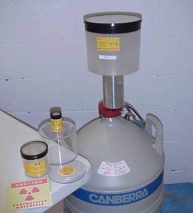 All 4
sources are then counted on the customer's detector at contact and at 10cm
[except for MB] for a total of 7 different acquisitions. Each source is carefully centered by placing
on a disc with concentric circles. The
10cm distance is created by placing the source on the hollow plastic cylinder
shown in the figure. For each of the 7
geometries, a LabSOCS efficiency calibration is generated using the to-be-delivered software. Each of the 7 spectra is then analyzed as an
"unknown". The reported
activity for each of the 13 energy lines is then compared to the
"true" decay-corrected activity from the source certificate, and a
report is then generated. This is the
process that happens when the customer orders the ISOXVRFY product. Table 2,
and Figure 2 from a typical ISOXVRFY customer report shows the results from one
of the 7 verification counts.
All 4
sources are then counted on the customer's detector at contact and at 10cm
[except for MB] for a total of 7 different acquisitions. Each source is carefully centered by placing
on a disc with concentric circles. The
10cm distance is created by placing the source on the hollow plastic cylinder
shown in the figure. For each of the 7
geometries, a LabSOCS efficiency calibration is generated using the to-be-delivered software. Each of the 7 spectra is then analyzed as an
"unknown". The reported
activity for each of the 13 energy lines is then compared to the
"true" decay-corrected activity from the source certificate, and a
report is then generated. This is the
process that happens when the customer orders the ISOXVRFY product. Table 2,
and Figure 2 from a typical ISOXVRFY customer report shows the results from one
of the 7 verification counts.
Figure 1 The 4 NIST traceable sources, centering ring
and 10cm spacer
|
Nuclide l |
Energy (keV) |
Meas Activity (LabSOCS eff) gammas/s |
Statistical uncertainty (1s) |
True Activity 06/12/2000 gammas/s |
Source uncertainty (1s) |
Meas/True |
rel. uncert (1s) |
Specified LabSOCS Uncert. |
|
|
Am-241 |
59.5 |
1342.5 |
0.17% |
1349.28 |
1.67% |
0.99 |
1.68% |
7.0% |
|
|
Cd-109 |
88 |
1087.5 |
0.21% |
1053.60 |
1.40% |
1.03 |
1.42% |
7.0% |
|
|
Co-57 |
122 |
490.4 |
0.36% |
466.09 |
1.57% |
1.05 |
1.61% |
7.0% |
|
|
*Ce-139* |
166 |
285.8 |
0.52% |
303.17 |
1.37% |
0.94 |
1.46% |
6.0% |
|
|
Hg-203 |
279 |
39.7 |
4.36% |
37.60 |
1.37% |
1.05 |
4.57% |
6.0% |
|
|
Sn-113 |
392 |
322.0 |
0.71% |
298.87 |
1.33% |
1.08 |
1.51% |
6.0% |
|
|
Cs-137 |
662 |
1247.5 |
0.42% |
1130.09 |
1.47% |
1.10 |
1.53% |
4.3% |
|
|
Mn-54 |
835 |
1565.2 |
0.41% |
1457.65 |
1.67% |
1.07 |
1.72% |
4.3% |
|
|
*Y-88* |
898 |
622.6 |
0.81% |
678.58 |
1.50% |
0.92 |
1.70% |
4.3% |
|
|
Zn-65 |
1115 |
1225.8 |
0.89% |
1178.53 |
1.67% |
1.04 |
1.89% |
4.3% |
|
|
*Co-60* |
1173 |
1855.3 |
0.43% |
1970.33 |
1.47% |
0.94 |
1.53% |
4.3% |
|
|
*Co-60* |
1332 |
1833.6 |
0.60% |
1982.94 |
1.53% |
0.92 |
1.65% |
4.3% |
|
|
*Y-88* |
1836 |
630.9 |
0.82% |
711.98 |
1.37% |
0.89 |
1.59% |
4.3% |
|
|
*Activities of Ce-139, Co-60, and Y-88 are
underestimated because of gamma ray cascade summing losses. The beaker file used in the LabSOCS calculations is FILTER.BKR. The diameter of the source matrix used in
LabSOCS calculations is 48 mm. |
|||||||||
Table 2 Results from analyzing reference source as
unknown (1 of 7)
From the results presented in the plots and tables, one
can observe that the measured activities of Co-60, Y-88, and in some cases,
Ce-139, are lower than their true activities [shown by the open circles in
Figure 2]. This is because of gamma ray cascade summing (or true coincidence
summing) losses in these nuclide measurements. The severity of cascade summing
errors is dependent upon the decay scheme of a given nuclide and the total
efficiency of the measurement geometry. The higher the total efficiency, the
greater is the loss due to cascade summing. In other words, cascade summing
losses will be more severe at smaller source-detector distances and with larger
detectors. The detector shown here is a
rather small one [25%], but the cascade summing errors are very significant,
approximately 10%. The datapoints in
Figure 2 with the open circles are those with cascade summing.
While Co-60 and Y-88 are will known cascade summing
emitters, the sources used in the verification tests also contain Ce-139. The energy of the principal gamma ray
emitted from the decay of Ce-139 is165 keV. This gamma ray undergoes true
coincidence summing with low energy X-rays emitted from Ce-139. Therefore,
cascade summing losses for Ce-139 are observable primarily in the case of
measurements with low energy detectors [as is the case here] because of the absence of the germanium dead-layer.
Nuclides and geometries where cascade summing is a major contributor to the
efficiency bias are not included in the bias calculation in the ISOXVRFY
report, but they will be used for future reports to evaluate the quality of the
cascade summing software. Canberra
Industries has developed a patented algorithm that corrects for cascade summing
effects. This algorithm and the supporting software will be incorporated into
Genie 2000 Version 2.0.
The data from the 7 individual count tables are then
grouped and summarized in a final table in the customer's report, as shown in
Table 3, for a typical detector. The
purpose of this table is to give the estimated overall performance and compare
it to the Validation Document's estimated performance.
|
ISOXVRFY |
Data
< 150 keV |
Data 150 - 400 keV |
Data > 400 keV |
|||||||||
|
Geometry |
Meas/True Ratio
(avg) |
Bias |
LabSOCS unc
(1s) |
Meas/True Ratio
(avg) |
Bias |
LabSOCS unc
(1s) |
Meas/True Ratio
(avg) |
Bias |
LabSOCS unc
(1s) |
|||
|
|
||||||||||||
|
Filter
Paper |
1.03 |
2.6% |
7.0% |
1.07 |
6.6% |
6.0% |
1.07 |
7.3% |
4.3% |
|||
|
(close) |
|
|
|
|
|
|
|
|
|
|||
|
Filter
Paper |
0.97 |
-2.7% |
7.0% |
1.06 |
6.5% |
6.0% |
1.02 |
1.7% |
4.3% |
|||
|
(far) |
|
|
|
|
|
|
|
|
|
|||
|
20mL
Cyl. |
0.92 |
-7.9% |
7.0% |
0.99 |
-0.6% |
6.0% |
0.98 |
-1.7% |
4.3% |
|||
|
(close) |
|
|
|
|
|
|
|
|
|
|||
|
20mL
Cyl. |
1.02 |
1.6% |
7.0% |
1.03 |
3.3% |
6.0% |
1.05 |
5.4% |
4.3% |
|||
|
(far) |
|
|
|
|
|
|
|
|
|
|||
|
350mL
Cyl. |
0.94 |
-6.3% |
7.0% |
0.99 |
-0.7% |
6.0% |
0.98 |
-2.5% |
4.3% |
|||
|
(close) |
|
|
|
|
|
|
|
|
|
|||
|
350mL
Cyl. |
1.00 |
-0.1% |
7.0% |
1.09 |
9.3% |
6.0% |
1.04 |
3.7% |
4.3% |
|||
|
(far) |
|
|
|
|
|
|
|
|
|
|||
|
2.8L
Marinelli |
0.95 |
-5.1% |
7.0% |
1.03 |
3.2% |
6.0% |
1.00 |
0.1% |
4.3% |
|||
|
(close) |
|
|
|
|
|
|
|
|
|
|||
|
Average (all) |
0.97 |
|
|
1.04 |
|
|
1.02 |
|
|
|||
|
% Std Dev |
4.4% |
|
|
3.9% |
|
|
4.4% |
|
|
|||
Average Bias |
3.8% |
|
|
4.3% |
|
|
3.2% |
|
||||
|
LabSOCS Uncertainty (1s) this det |
4.1% |
|
|
1.1% |
|
|
4.0% |
|||||
Table 3 Summary data for all 7 counts for a typical
detector
Within Table 3, the results for each geometry are grouped
into three energy regimes; (i) less than 150 keV, (ii) 150-400 keV and (iii)
greater than 400 keV. For each energy regime, the following results are
presented.
· The
average value of the measured to true activity ratio, for nuclides within the
energy range
· The
bias in the ISOCS efficiency of this detector, obtained by calculating the
deviation of the average value of the ratio from its true mean, the true mean
being unity. Nuclides exhibiting cascade summing are not included.
· The
estimated uncertainty in LabSOCS efficiencies, derived from Canberra's
validation test database, for a group of detectors.
· The
average value of the measured to true activity ratio for a given energy range,
computed by pooling together the ratios from all seven geometries.
· The
standard deviation of the ratios for a given energy range, computed by pooling
together the ratios from all seven geometries.
· The
average uncertainty in LabSOCS efficiencies for this specific detector,
computed as the difference between the standard deviation of the ratios and the
measurement uncertainties.
· The
LabSOCS uncertainty for this detector, as calculated in the same manner as
described in the Validation and Internal Consistency document
It is hoped that the ISOXVRFY report will be helpful to
the customer proving to himself and to others that efficiencies created using
the LabSOCS software will give correct analysis results on his system, and that
laboratory-specific testing can be minimized and the software can then be
quickly used for production counting.
All of the data from this process are also summarized
and reviewed periodically as a quality control measure, to improve the process,
and to add to the validation database.
For this document, we have summarized the first 13 detectors that have
been completed using the standard production process and present that data in
Table 4.
|
Summary
of first 13 ISOXVRFY detectors |
|||
|
|
<150 keV |
150-400 keV |
>400 keV |
|
Average Bias |
1.0% |
1.9% |
-1.9% |
|
Average |Bias| |
5.5% |
5.7% |
4.6% |
|
sd from ISOXVRFY |
5.1% |
5.1% |
4.2% |
|
sd from Validation Doc |
7.1% |
6.0% |
4.3% |
Table 4 Summary of
accuracy and precision from first 13 detectors
This data indicates that the performance of the new
detector characterization process is about the same before for high energies,
but better than before at medium and low energies. This are the first detectors
done with this new process, and some improvement was expected, however
detectors being produced today should be even better. Observations of the full data set show that the later ones are
better than the early ones. And, we are
about to incorporate some additional steps to the detector characterization
process which should even further reduce the uncertainty at these close-up
distances.
But, even as this data currently stands [4-5% sd], it is
probably as good or better than most source based calibrations. Source-based
calibrations, even using these carefully manufactured sources had
problems. The 51mm source actually was
48mm in effective diameter, which is a 4% difference in efficiency. Two "identically manufactured"
source sets were about 2-3% different from each other. The Hg-203 activity on a few [but not all]
of the sources keeps "changing" with time, at a rate inconsistent
with the half-life, and appears to be 10-20% different than the correct
activity. Even though the sources are
in an epoxy matrix, apparently the Hg being redistributed as the source
ages. And, there are the 10% [20-30%
for larger detectors] due to cascade summing if Y-88, Ce-139, Co-60, or Eu-152
are used without correction. So, the 4-5% sd from the LabSOCS process certainly
seems acceptable for most laboratory sample assay processes, and is certainly
more convenient, and quick than source-based calibrations.