Flux Terms

All of the terms in Equation 6 are evaluated in terms of known quantities, or in terms of the unknown $\Phi$, except for the flux term. To effect closure, the flux vector across each face of the cell, $\mbox{$\stackrel{^{\mathstrut}\smash{\longrightarrow}}{F_f^{n+1}}$}$, must be expressed in terms of $\Phi^{{n+1}}_{}$.

Evaluating the flux equation, Equation 3, at a particular face gives $$\mbox{$\stackrel{^{\mathstrut}\smash{\longrightarrow}}{F_f^{n... ...x{$\stackrel{^{\mathstrut}\smash{\longrightarrow}}{J_f}$} \; .$$
The flux source, $\mbox{$\stackrel{^{\mathstrut}\smash{\longrightarrow}}{J_f}$}$, is known. The diffusion coefficient, D_{c, f}, is known within a cell, but may be discontinuous at the cell face. In general, one cannot evaluate a gradient by taking differences across a material interface because the gradient is discontinuous along the interface. It is often assumed that one can take differences across a material discontinuity if one uses a proper average of the two diffusion coefficients on each side of the discontinuity. However, it will be shown that this is possible only on orthogonal meshes. To avoid taking differences across material discontinuities, an intensity unknown is added to each cell face. The interface flux is then evaluated using two independent differences, with each difference being constructed solely from unknowns from a single cell. An equation for each interface intensity is obtained by requiring these independent differences to yield the same flux.

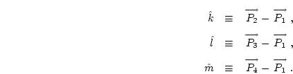
Actual expressions for the gradient in non-orthogonal coordinate systems will now be considered. The values of $\Phi$ at four non-planar points are necessary and sufficient to determine the gradient. Since the mesh is unstructured, a unique coordinate system will be defined for each cell. Any four non-planar points ( $\mbox{$\stackrel{^{\mathstrut}\smash{\longrightarrow}}{P_1}$}$,$\mbox{$\stackrel{^{\mathstrut}\smash{\longrightarrow}}{P_2}$}$,$\mbox{$\stackrel{^{\mathstrut}\smash{\longrightarrow}}{P_3}$}$,$\mbox{$\stackrel{^{\mathstrut}\smash{\longrightarrow}}{P_4}$}$) define a local coordinate system (see Figure 3) in

Figure 3: Coordinate system defined by four non-planar points.

terms of three vectors,

$$\begin{eqnarray}\html{eqn17} \hat{k} & \equiv & \mbox{$\stackrel{^{\mathstrut}\... ...krel{^{\mathstrut}\smash{\longrightarrow}}{P_1}$} \; . \nonumber \end{eqnarray}$$

The coordinates of the four points in $\left(\vphantom{ k,l,m }\right.$k, l, m$\left.\vphantom{ k,l,m }\right)$-space are defined to be $\mbox{$\stackrel{^{\mathstrut}\smash{\longrightarrow}}{{\cal P}_1}$}$ $\equiv$ (0, 0, 0)^T, $\mbox{$\stackrel{^{\mathstrut}\smash{\longrightarrow}}{{\cal P}_2}$}$ $\equiv$ (1, 0, 0)^T, $\mbox{$\stackrel{^{\mathstrut}\smash{\longrightarrow}}{{\cal P}_3}$}$ $\equiv$ (0, 1, 0)^T, and $\mbox{$\stackrel{^{\mathstrut}\smash{\longrightarrow}}{{\cal P}_4}$}$ $\equiv$ (0, 0, 1)^T. A Jacobian matrix converts between the $\left(\vphantom{ k,l,m }\right.$k, l, m$\left.\vphantom{ k,l,m }\right)$ coordinate system and the $\left(\vphantom{ x,y,z }\right.$x, y, z$\left.\vphantom{ x,y,z }\right)$ coordinate system: $$\left[ \begin{array}{c} P^x \ [1em] P^y \ [1em] P^z \e... ...m] {\cal P}^l \ [1em] {\cal P}^m \end{array} \right] \; .$$
which is represented as: $$\mbox{$\stackrel{^{\mathstrut}\smash{\longrightarrow}}{P}$} -... ...\stackrel{^{\mathstrut}\smash{\longrightarrow}}{\cal P}$} \; .$$

Note that an equally valid inverse transformation from the $\left(\vphantom{ x,y,z }\right.$x, y, z$\left.\vphantom{ x,y,z }\right)$ coordinate system to the $\left(\vphantom{ k,l,m }\right.$k, l, m$\left.\vphantom{ k,l,m }\right)$ coordinate system could have been used, with a Jacobian matrix equal to J^-1. However, since the four points are located along the axes in (k, l, m)-space, but not in (x, y, z)-space, it is easier to take the derivatives needed for the forward Jacobian than the reverse Jacobian:

$$\begin{eqnarray}\html{eqn22} \mathbf{J} & \! \! = \! & \left[ \begin{array}{ccc... ...}{ccc} \hat{k} & \hat{l} & \hat{m} \\ \end{array} \right] \; . \end{eqnarray}$$

Returning to the consideration of the gradient term and expanding the k, l and m derivatives of $\Phi$ using the chain rule yields

$$\begin{eqnarray}\html{eqn25} \left[ \begin{array}{c} \frac{\partial \Phi}{\par... ...ackrel{^{\mathstrut}\smash{\longrightarrow}}{\nabla}$}$}\Phi \; , \end{eqnarray}$$

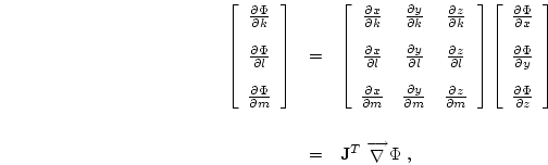
or, solving for $\mbox{$\mbox{$\stackrel{^{\mathstrut}\smash{\longrightarrow}}{\nabla}$}$}$$\Phi$ and inserting the derivative definitions, $$\mbox{$\mbox{$\stackrel{^{\mathstrut}\smash{\longrightarrow}}... ...\Phi_1 \ [1em] \Phi_4 - \Phi_1 \\ \end{array} \right] \; .$$

This method of representing gradients is exact for linear functions, but only approximate for higher order functions.

Four points are not the only way to determine a gradient, for instance, six points that form three lines intersecting in a single point can also be used. A six points gradient is actually used to determine the fluxes on the faces of the cell. If a point (and therefore an unknown $\Phi$) is placed in the center of each face, the three lines formed by connecting opposing faces all intersect at the cell center. A single Jacobian matrix per cell is then sufficient to determine the necessary gradients.

If the vectors connecting the face centers of opposite faces are denoted $\mbox{$\stackrel{^{\mathstrut}\smash{\longrightarrow}}{J_k}$}$, $\mbox{$\stackrel{^{\mathstrut}\smash{\longrightarrow}}{J_l}$}$, and $\mbox{$\stackrel{^{\mathstrut}\smash{\longrightarrow}}{J_m}$}$ for the k, l, and m directions (see Figure 4), then the Jacobian matrix is given by

Figure 4: Coordinate system defined by three intersecting lines.

$$\mathbf{J} = \left[ \begin{array}{ccc} \mbox{$\stackrel{^{\... ...}\smash{\longrightarrow}}{J_m}$} \\ \end{array} \right] \; ,$$
and the inverse transpose matrix is

$$\begin{eqnarray}\html{eqn39} \lefteqn{\mathbf{J}^{-T} =} \\ & & \hspace{-3ex... ...htarrow}}{J_l}$} \right) \\ \end{array} \right] \nonumber \; . \end{eqnarray}$$

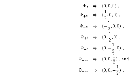
The values for the k, l and m derivatives of $\Phi$ have yet to be defined. These are defined in terms of the seven unknown $\Phi$'s in each cell. If the origin is placed at the center of the cell, then the locations of the unknown $\Phi$'s in (k, l, m)-space are

$$\begin{eqnarray}\html{eqn41} \Phi_c & \Rightarrow & (0,0,0) \; , \nonumber \\ ... ...\\ \Phi_{-m} & \Rightarrow & (0,0,-\frac{1}{2}) \; , \nonumber \end{eqnarray}$$

where the faces are denoted + k, - k, + l, - l, + m and - m. Along any particular direction there are three ways to determine a derivative. For example, in the k direction, the k derivative of $\Phi$ can be determined via

$$\begin{eqnarray}\html{eqn42} \frac{\partial \Phi}{\partial k} & = & \frac{\Phi_... ...\right)} = 2\left( \Phi_{c} - \Phi_{-k} \right) \; . \nonumber \end{eqnarray}$$

The first definition uses a full-cell difference, whereas the second and third definitions use a half-cell difference. Each of these definitions will be used depending on which direction and which face is being considered.

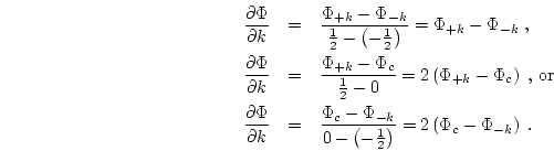
The gradient must be determined for each face of the cell. Each face must have definitions for all of the k, l and m derivatives. For a given face, the direction which is perpendicular to the face is called the major direction, because it is the only direction for which the derivative is non-zero if the cell is orthogonal, and it is usually the main contributor to the flux across the face. The other directions are called the minor directions for that face.

To compute the gradient for a face, full-cell derivatives are used for the minor directions. The half-cell derivative which involves the face in question is used for the major direction. For example, for the + k face the major direction is the k direction, and the minor directions are the l and m directions. The gradient for the + k face is represented by the cell value for the J^-T matrix multiplied by the k, l and m derivative vector for that face: $$\mbox{$\stackrel{^{\mathstrut}\smash{\longrightarrow}}{F_{+k}... ...{$\stackrel{^{\mathstrut}\smash{\longrightarrow}}{J_{c,+k}}$}$$
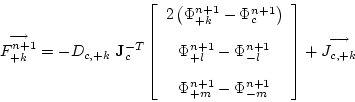
Figure 5 shows the stencil for each face gradient that is given by this method.

Figure 5: Stencil for the + k face gradient, shown with a dotted blue line.

This completes the discretization of the conservation equation, Equation 2. When all of the face gradients have been defined and substituted in, the conservation equation has terms for all of the seven unknowns within the cell and has no terms involving any unknowns that are not within the cell.